带单位,写 t > 0 t>0 t > 0 When solving Thevenin equialent/Norton equialent, determine the positive / negative voltage.
If there is a voltage source across the resistor we want to obtain the Thevein equivalent(or there is a current source through the branch), we can only find V t h V_{th} V t h I N I_{N} I N R t h R_{th} R t h R N R_{N} R N 0 0 0 ∞ \infty ∞
power is different from energy
saturate 饱和
DC 直流
ideal transformer: When the voltage is not given in the problem, it can be set by yourself.
fraction 分数 / 比例
w = 2 π f w=2\pi f w = 2 π f Note the positive and negative of voltage and current!!!
DC circuits
A branch ( Number b b b n n n l l l n − 1 n-1 n − 1
b = l + n − 1 b=l+n-1 b = l + n − 1 R 1 = R b R c R a + R b + R c R_{1}=\frac{R_{b}R_{c} }{R_{a}+R_{b}+R_{c} } R 1 = R a + R b + R c R b R c (自己在对面,两面夹击,除以所有)
R a = R 1 R 2 + R 2 R 3 + R 3 R 1 R 1 R_{a}=\frac{ {R_{1}R_{2}+R_{2}R_{3}+R_{3}R_{1} }}{R_{1} } R a = R 1 R 1 R 2 + R 2 R 3 + R 3 R 1 (所有相乘,除以自己,得到对面)
[ G 11 G 12 ⋯ G 1 N G 21 G 22 ⋯ G 2 N ⋮ ⋮ ⋮ ⋮ G N 1 G N 2 ⋯ G N N ] [ v 1 v 2 ⋮ v N ] = [ i 1 i 2 ⋮ i N ] \left[ \begin{matrix} {G_{1 1} } & {G_{1 2} } & {\cdots} & {G_{1 N} } \\ {G_{2 1} } & {G_{2 2} } & {\cdots} & {G_{2 N} } \\ {\vdots} & {\vdots} & {\vdots} & {\vdots} \\ {G_{N 1} } & {G_{N 2} } & {\cdots} & {G_{N N} } \\ \end{matrix} \right] \left[ \begin{matrix} {v_{1} } \\ {v_{2} } \\ {\vdots} \\ {v_{N} } \\ \end{matrix} \right]=\left[ \begin{matrix} {i_{1} } \\ {i_{2} } \\ {\vdots} \\ {i_{N} } \\ \end{matrix} \right] G 11 G 21 ⋮ G N 1 G 12 G 22 ⋮ G N 2 ⋯ ⋯ ⋮ ⋯ G 1 N G 2 N ⋮ G NN v 1 v 2 ⋮ v N = i 1 i 2 ⋮ i N G k k G_{kk} G kk G k j = G j k G_{kj}=G_{jk} G kj = G jk v k v_{k} v k i k i_{k} i k
[ R 11 R 12 ⋯ R 1 N R 21 R 22 ⋯ R 2 N ⋮ ⋮ ⋮ ⋮ R N 1 R N 2 ⋯ R N N ] [ i 1 i 2 ⋮ i N ] = [ v 1 v 2 ⋮ v N ] \left[ \begin{matrix} {R_{1 1} } & {R_{1 2} } & {\cdots} & {R_{1 N} } \\ {R_{2 1} } & {R_{2 2} } & {\cdots} & {R_{2 N} } \\ {\vdots} & {\vdots} & {\vdots} & {\vdots} \\ {R_{N 1} } & {R_{N 2} } & {\cdots} & {R_{N N} } \\ \end{matrix} \right] \left[ \begin{matrix} {i_{1} } \\ {i_{2} } \\ {\vdots} \\ {i_{N} } \\ \end{matrix} \right]=\left[ \begin{matrix} {v_{1} } \\ {v_{2} } \\ {\vdots} \\ {v_{N} } \\ \end{matrix} \right] R 11 R 21 ⋮ R N 1 R 12 R 22 ⋮ R N 2 ⋯ ⋯ ⋮ ⋯ R 1 N R 2 N ⋮ R NN i 1 i 2 ⋮ i N = v 1 v 2 ⋮ v N R k k R_{kk} R kk R k j = R j k R_{kj}=R_{jk} R kj = R jk k k k j j j i k i_{k} i k k k k v k v_{k} v k k k k
Super Node & Super Mesh
Network theorems
Superposition principle
Source transformation
Thevenins(open-circuit voltage)/Norton(short-circuit current) theorems
R N = R T h R_{N}=R_{Th} R N = R T h I N = V T h R T h I_{N}=\frac{V_{Th} }{R_{Th} } I N = R T h V T h R L = R T h R_{L}=R_{Th} R L = R T h
Wheatstone bridge
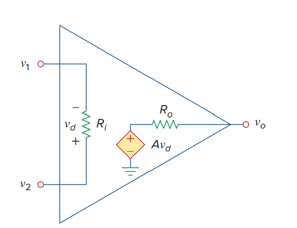
op amp equivalent circuit
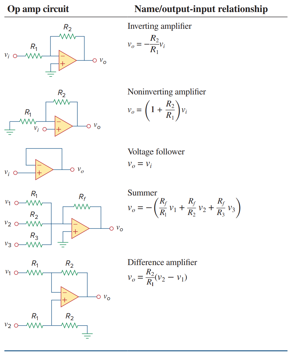
basic op amp circuits
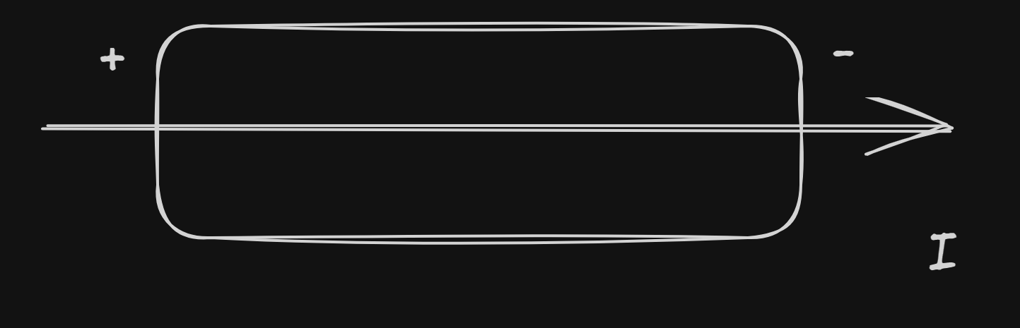
With an ideal op-amp, the output voltage changes immediately when the voltage at the input changes, and for this reason the current can potentially reach infinite values.
current through a capacitor---like conductors---voltage can't change instantly
i = C d v d t i=C \frac{dv}{dt} i = C d t d v
voltage across an inductor---like resistors---current can't change instantly
v = L d i d t v=L \frac{di}{dt} v = L d t d i
energy stored in a capacitor 1 2 C v 2 \frac{1}{2}Cv^2 2 1 C v 2 1 2 L i 2 \frac{1}{2}Li^2 2 1 L i 2 1 2 L ( i ( t ) 2 − i ( 0 ) 2 ) \frac{1}{2}L(i(t)^2-i(0)^2) 2 1 L ( i ( t ) 2 − i ( 0 ) 2 ) Please note that Thevenin equivalent circuits do not generally exist for circuits involving capacitors and resistors. D-W/W-D of capacitor & inductor: find the inverse of capacitor
Thevenin equivalent of circuits involving capacitors and resistors, we can get C T h C_{Th} C T h
For capacitors: v ( 0 ) + = v ( 0 ) − v(0)^+=v(0)^- v ( 0 ) + = v ( 0 ) −
For inductors: i ( 0 ) + = i ( 0 ) − i(0)^+=i(0)^- i ( 0 ) + = i ( 0 ) −
Complete response:
C o m p l e t e r e s p o n s e = n a t u r a l r e p o n s e + f o r c e d r e s p o n s e = t r a n s i e n t r e s p o n s e + s t e a d y − s t a t e r e s p o n s e Complete\ response=natural\ reponse+forced\ response=transient\ response+steady-state \ response C o m pl e t e res p o n se = na t u r a l re p o n se + f orce d res p o n se = t r an s i e n t res p o n se + s t e a d y − s t a t e res p o n se
τ \tau τ τ = R C \tau=RC τ = RC R L RL R L τ = L R \tau=\frac{L}{R} τ = R L Singularity functions:
unit step function u ( t ) u(t) u ( t ) u ( t ) = { 0 , t < 0 1 , t > 0 u ( t )=\left\{\begin{matrix} {0,} & {\qquad t < 0} \\ {1,} & {\qquad t > 0} \\ \end{matrix} \right. u ( t ) = { 0 , 1 , t < 0 t > 0
unit impulse function: δ ( t ) = { 0 , t < 0 U n d e f i n e d , t = 0 0 , t > 0 \delta( t )=\begin{cases} {0,} & {\qquad t < 0} \\ {\mathrm{U n d e f i n e d},} & {\qquad t=0} \\ {0,} & {\qquad t > 0} \\ \end{cases} δ ( t ) = ⎩ ⎨ ⎧ 0 , Undefined , 0 , t < 0 t = 0 t > 0 Meaningful only when integrating
unit ramp function: r ( t ) = { 0 , t ≤ 0 t , t ≥ 0 r ( t )=\left\{\begin{matrix} {0,} & {\qquad t \leq0} \\ {t,} & {\qquad t \geq0} \\ \end{matrix} \right. r ( t ) = { 0 , t , t ≤ 0 t ≥ 0
wave representation: not to have negative coefficients in singularity functions and Note the coefficients on the axes τ = R C / L R \tau=RC / \frac{L}{R} τ = RC / R L step response(short-cut approach)
x ( t ) = x ( ∞ ) + [ x ( t 0 + ) − x ( ∞ ) ] e − ( t − t 0 ) / τ x ( t )=x ( \infty)+[ x ( t_{0}^{+} )-x ( \infty) ] e^{-( t-t_{0} ) / \tau} x ( t ) = x ( ∞ ) + [ x ( t 0 + ) − x ( ∞ )] e − ( t − t 0 ) / τ
Short-cut approach can only be applied to voltage across capacitor. Sometimes can't use this method(in op amp), so we need to use straightforward approach. finding initial values: looking at voltage across the capacitors and current through the inductors, and get other values
source free RLC series:
quadratic equation: s 2 + R L s + 1 L C = 0 s^2+\frac{R}{L}s+\frac{1}{LC}=0 s 2 + L R s + L C 1 = 0
natural frequencies :
s 1 = − α + α 2 − w 0 2 s_{1}=-\alpha+\sqrt{ \alpha^2-w_{0}^2 } s 1 = − α + α 2 − w 0 2 s 2 = − α − α 2 − w 0 2 s_{2}=-\alpha-\sqrt{ \alpha^2-w_{0}^2 } s 2 = − α − α 2 − w 0 2
neper frequency: α = R 2 L \alpha=\frac{R}{2L} α = 2 L R resonant frequency / undamped natural frequency : w 0 = 1 L C w_{0}=\frac{1}{\sqrt{ LC } } w 0 = L C 1 s 2 + 2 a s + w 0 2 = 0 s^2+2as+w_{0}^2=0 s 2 + 2 a s + w 0 2 = 0 i ( t ) = A 1 e s 1 t + A 2 e s 2 t i(t)=A_{1}e^{ s_{1}t }+A_{2}e^{ s_{2}t } i ( t ) = A 1 e s 1 t + A 2 e s 2 t A 1 A_{1} A 1 A 2 A_{2} A 2 i ( 0 ) i(0) i ( 0 ) d i ( 0 ) d t \frac{di(0)}{dt} d t d i ( 0 )
three types of solutions
overdamped case α > w 0 \alpha>w_{0} α > w 0
decays and approaches zero as it increases
i ( t ) = A 1 e s 1 t + A 2 e s 2 t i(t)=A_{1}e^{ s_{1}t }+A_{2}e^{ s_{2}t } i ( t ) = A 1 e s 1 t + A 2 e s 2 t
critically damped case α = w 0 \alpha=w_{0} α = w 0 s 1 = s 2 = − α s_{1}=s_{2}=-\alpha s 1 = s 2 = − α
i ( t ) = ( A 2 + A 1 t ) e − α t i(t)=(A_{2}+A_{1}t)e^{ -\alpha t } i ( t ) = ( A 2 + A 1 t ) e − α t
underdamped case α < w 0 \alpha<w_{0} α < w 0
s 1 = − α + j w d s_{1}=-\alpha+jw_{d} s 1 = − α + j w d s 2 = − α − j w d s_{2}=-\alpha-jw_{d} s 2 = − α − j w d w d = w 0 2 − α 2 w_{d}=\sqrt{ w_{0}^2-\alpha^2 } w d = w 0 2 − α 2 i ( t ) = e − α t ( B 1 cos w d t + B 2 sin w d t ) i(t)=e^{ -\alpha t }(B_{1}\cos w_{d}t+B_{2}\sin w_{d}t) i ( t ) = e − α t ( B 1 cos w d t + B 2 sin w d t )
source free RLC parallel
α = 1 2 R C \alpha=\frac{1}{2RC} α = 2 RC 1 w 0 = 1 L C w_{0}=\frac{1}{\sqrt{ LC } } w 0 = L C 1 solving the constant by getting v ( 0 ) v(0) v ( 0 ) d v ( 0 ) d t \frac{dv(0)}{dt} d t d v ( 0 )
step response: v s s / i s s ( t ) = v / i ( ∞ ) = V s / I s v_{ss} / i_{ss}(t)=v / i(\infty)=V_{s} / I_{s} v ss / i ss ( t ) = v / i ( ∞ ) = V s / I s
x ( t ) = x t ( t ) + x s s ( t ) x(t)=x_{t}(t)+x_{ss}(t) x ( t ) = x t ( t ) + x ss ( t )
Simple method: Simplify as much as possible to RLC series or RLC parallel or directly use Thevenins theroem.
AC circuits
Fundamentals
V m V_{m} V m cos ( w t + ϕ ) → ∠ ϕ \cos(wt+\phi)\to \angle \phi cos ( wt + ϕ ) → ∠ ϕ sin ( w t + ϕ ) → ∠ ϕ − 9 0 ∘ \sin(wt+\phi)\to \angle{\phi-90^\circ} sin ( wt + ϕ ) → ∠ ϕ − 9 0 ∘ d v d t ⇔ j w V \frac{dv}{dt} \Leftrightarrow jwV d t d v ⇔ j w V ∫ v d t ⇔ V j w \int v \, dt \Leftrightarrow \frac{V}{jw} ∫ v d t ⇔ j w V inductor: V = j w L I V=jwLI V = j w L I I I I V V V
capacitor: V = I j w C V=\frac{I}{jwC} V = j wC I V V V I I I
Y = G + j B = 1 R + j X Y=G+jB=\frac{1}{R+jX} Y = G + j B = R + j X 1 other: Y − Δ Y-\Delta Y − Δ
superposition theorem: different frequencies
Power analysis
Be careful to distinguish between amplitude and RMS values!
instantaneous power: p ( t ) = v ( t ) i ( t ) p(t)=v(t)i(t) p ( t ) = v ( t ) i ( t )
average power: P = 1 2 V m I m cos ( θ v − θ i ) P=\frac{1}{2}V_{m}I_{m}\cos(\theta_{v}-\theta_{i}) P = 2 1 V m I m cos ( θ v − θ i )
θ v = θ i \theta_{v}=\theta_{i} θ v = θ i P = 1 2 V m I m = 1 2 I m 2 R = 1 2 ∣ I ∣ 2 R P=\frac{1}{2}V_{m}I_{m}=\frac{1}{2}I_{m}^2R=\frac{1}{2}\mid I\mid^2R P = 2 1 V m I m = 2 1 I m 2 R = 2 1 ∣ I ∣ 2 R
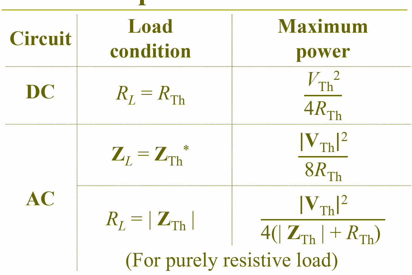
maximum average power transfer (so a factor of 1 2 \frac{1}{2} 2 1
Z L = Z T h ∗ Z_{L}=Z^*_{Th} Z L = Z T h ∗
when X L = 0 X_{L}=0 X L = 0 R L = ∣ Z T h ∣ R_{L}=\mid Z_{Th}\mid R L =∣ Z T h ∣
rms: X r m s = 1 T ∫ 0 T x 2 d t X_{rms}=\sqrt{ \frac{1}{T}\int _{0}^T \,x^2 dt } X r m s = T 1 ∫ 0 T x 2 d t
I r m s = I m 2 I_{rms}=\frac{I_{m} }{\sqrt{ 2 } } I r m s = 2 I m V r m s = V m 2 V_{rms}=\frac{V_{m} }{\sqrt{ 2 } } V r m s = 2 V m if V / I V / I V / I c + d sin … c+d\sin \dots c + d sin … V r m s / I r m s = c 2 + d 2 2 V_{rms} / I_{r ms}=\sqrt{ c^2+\frac{d^2}{2} } V r m s / I r m s = c 2 + 2 d 2
apparent power(VA):
S = 1 2 V I ∗ S=\frac{1}{2}VI^* S = 2 1 V I ∗ S = V r m s I r m s ∗ S=V_{rms}I^*_{rms} S = V r m s I r m s ∗ S = I r m s 2 Z = V r m s 2 Z ∗ S=I^2_{rms}Z=\frac{V^2_{rms} }{Z^*} S = I r m s 2 Z = Z ∗ V r m s 2 When answering the question, S should be written in the form P + j Q P+jQ P + j Q Q Q Q
power factor p f = P S = cos ( θ v − θ i ) pf=\frac{P}{S}=\cos(\theta_{v}-\theta_{i}) p f = S P = cos ( θ v − θ i )
leading: current leads voltage
lagging: voltage leads current
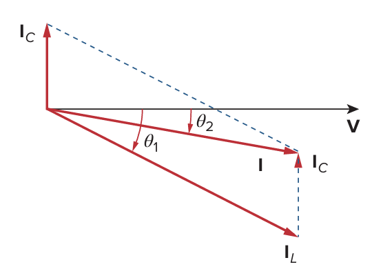
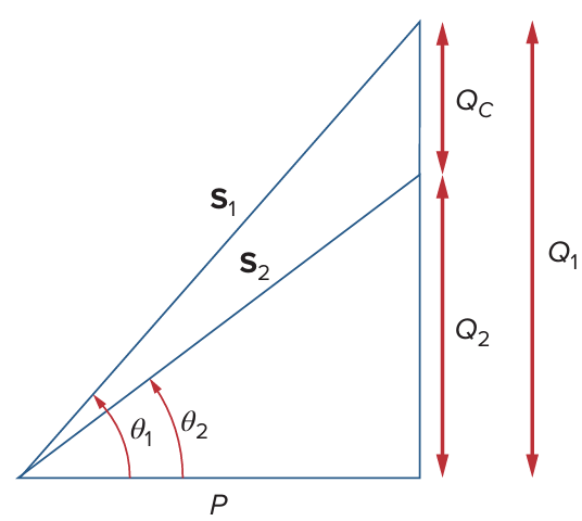
power factor correction
phasor diagram:
power factor correction
C = Q c w 2 V r m s = P ( tan θ 1 − tan θ 2 ) w V r m s 2 C=\frac{Q_{c} }{w^2V_{r ms} }=\frac{P(\tan\theta_{1}-\tan\theta_{2})}{wV^2_{rms} } C = w 2 V r m s Q c = w V r m s 2 P ( t a n θ 1 − t a n θ 2 ) Q L = V r m s 2 X L Q_{L}=\frac{V^2_{r ms} }{X_{L} } Q L �� = X L V r m s 2
reactive power: Q = I m ( S ) = I r m s 2 X = V r m s I r m s sin ( θ v − θ i ) Q=Im(S)=I^2_{r ms} X=V_{r ms}I_{r ms}\sin(\theta_{v}-\theta_{i}) Q = I m ( S ) = I r m s 2 X = V r m s I r m s sin ( θ v − θ i )
Q = 0 Q=0 Q = 0 Q < 0 Q<0 Q < 0 leading pf )Q > 0 Q>0 Q > 0 lagging pf )power triangle: using Q Q Q Q Q Q
∣ Z ∣ = R 2 + X 2 |Z|=\sqrt{ R^2+X^2 } ∣ Z ∣ = R 2 + X 2
Three-Phase Circuits
in three-phase circuits, V p V_{p} V p rms value of the phase voltages
phase sequence: time order in which voltage pass through their respective maximum values
positive: V a n , V b n , V c n V_{an},V_{bn},V_{cn} V an , V bn , V c n
negative: V a n , V b n , V c n V_{an},V_{bn},V_{cn} V an , V bn , V c n
phase xx: line-to-neutual xx
line xx: line-to-line xx
Y Y Y
V L = 3 V P V_{L}=\sqrt{ 3 }V_{P} V L = 3 V P V a b = 3 V a n ∠ 3 0 ∘ V_{ab}=\sqrt{ 3 }V_{an}\angle 30^\circ V ab = 3 V an ∠3 0 ∘
Δ \Delta Δ
I L = 3 I P I_{L}=\sqrt{ 3 }I_{P} I L = 3 I P I a = 3 I A B ∠ − 3 0 ∘ I_{a}=\sqrt{ 3 }I_{AB}\angle -30^\circ I a = 3 I A B ∠ − 3 0 ∘
power (remind to × 3 \times3 × 3
S = 3 S p = 3 V p I p ∗ = 3 I p 2 Z p = 3 V p 2 Z p ∗ S=3S_{p}=3V_{p}I_{p}^*=3I_{p}^2Z_{p}=\frac{3V_{p}^2}{Z_{p}^*} S = 3 S p = 3 V p I p ∗ = 3 I p 2 Z p = Z p ∗ 3 V p 2 Z p = Z p ∠ θ \mathbf{Z_{p} }=Z_{p}\angle\theta Z p = Z p ∠ θ S = 3 V p I p ∠ θ = 3 V L I L ∠ θ \mathbf{S}=3V_{p}I_{p}\angle\theta=\sqrt{ 3 }V_{L}I_{L}\angle \theta S = 3 V p I p ∠ θ = 3 V L I L ∠ θ
power loss of transmission lines in three-phase system and single-phase system
single-phase: I L = P L V L I_{L}=\frac{P_{L} }{V_{L} } I L = V L P L
P l o s s = 2 I L 2 R = 2 R P L 2 V L P_{loss}=2I_{L}^2R=2R \frac{P_{L}^2}{V_{L} } P l oss = 2 I L 2 R = 2 R V L P L 2
three-phase: I L = P L 3 V L I_{L}=\frac{P_{L} }{\sqrt{ 3 }V_{L} } I L = 3 V L P L
P l o s s = 3 I L 2 R = R P L 2 V L 2 P_{loss}=3I_{L}^2R=R \frac{P_{L}^2}{V_L^2} P l oss = 3 I L 2 R = R V L 2 P L 2
no need to get conjuction when doing Δ − Y \Delta-Y Δ − Y
Magnetically Coupled Circuits
Be careful with the dot convention!!!
voltage ratings of transformers are usually specified in rms values
mutual voltage(eg)
v 1 = M 12 d i 2 d t v_{1}=M_{12} \frac{di_{2} }{dt} v 1 = M 12 d t d i 2
M = k L 1 L 2 M=k\sqrt{ L_{1}L_{2} } M = k L 1 L 2 dot convention
enter the dotted terminal → \to →
leave the dotted terminal → \to →
induction in series
aiding connection: L = L 1 + L 2 + 2 M L=L_{1}+L_{2}+2M L = L 1 + L 2 + 2 M
opposing connection: L = L 1 + L 2 − 2 M L=L_{1}+L_{2}-2M L = L 1 + L 2 − 2 M
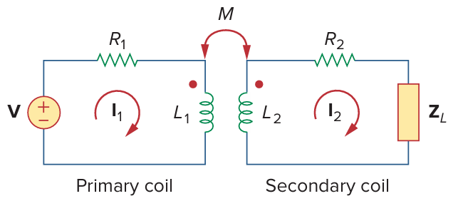
Transformer
From two KVL: Z i n = R 1 + j w L 1 + w 2 M 2 R 2 + j w L 2 + Z L Z_{in}=R_{1}+jwL_{1}+ \frac{ {w^2M^2} }{R_{2}+jwL_{2}+Z_{L} } Z in = R 1 + j w L 1 + R 2 + j w L 2 + Z L w 2 M 2
Z R = w 2 M 2 R 2 + j w L 2 + Z L Z_{R}=\frac{w^2M^2}{R_{2}+jwL_{2}+Z_{L} } Z R = R 2 + j w L 2 + Z L w 2 M 2
I-V relationships
[ V 1 V 2 ] = [ j ω L 1 j ω M j ω M j ω L 2 ] [ I 1 I 2 ] \left[ \begin{matrix} { {\bf V}_{1} } \\ { {\bf V}_{2} } \\ \end{matrix} \right]=\left[ \begin{matrix} {j \omega L_{1} } & {j \omega M} \\ {j \omega M} & {j \omega L_{2} } \\ \end{matrix} \right] \left[ \begin{matrix} { {\bf I}_{1} } \\ { {\bf I}_{2} } \\ \end{matrix} \right] [ V 1 V 2 ] = [ jω L 1 jω M jω M jω L 2 ] [ I 1 I 2 ]
change to T circuit:
[ V 1 V 2 ] = [ j ω ( L a + L c ) j ω L c j ω L c j ω ( L b + L c ) ] [ I 1 I 2 ] \left[ \begin{array} {c} { {\mathrm{V}_{1} }} \\ { {\mathrm{V}_{2} }} \\ \end{array} \right]=\left[ \begin{array} {c c} { {j \omega( L_{a}+L_{c} )} } & { {j \omega L_{c} }} \\ { {j \omega L_{c} }} & { {j \omega( L_{b}+L_{c} )} } \\ \end{array}\right] \left[ \begin{array} {c} { {\mathrm{I}_{1} }} \\ { {\mathrm{I}_{2} }} \\ \end{array} \right] [ V 1 V 2 ] = [ jω ( L a + L c ) jω L c jω L c jω ( L b + L c ) ] [ I 1 I 2 ] L a = L 1 − M L_{a}=L_{1}-M L a = L 1 − M L b = L 2 − M L_{b}=L_{2}-M L b = L 2 − M L c = M L_{c}=M L c = M
change to Π \Pi Π
[ I 1 I 2 ] = [ 1 j ω L A + 1 j ω L C − 1 j ω L C − 1 j ω L C 1 j ω L B + 1 j ω L C ] [ V 1 V 2 ] \left[ \begin{array} {c} { {\mathbf{I}_{1} }} \\ { {\mathbf{I}_{2} }} \end{array} \right]=\left[ \begin{array} {c c} { {\frac{1} {j \omega L_{A} }+\frac{1} {j \omega L_{C} }} } & { {-\frac{1} {j \omega L_{C} }} } \\ { {-\frac{1} {j \omega L_{C} }} } & { {\frac{1} {j \omega L_{B} }+\frac{1} {j \omega L_{C} }} } \\ \end{array} \right] \left[ \begin{array} {c} { {\mathbf{V}_{1} }} \\ { {\mathbf{V}_{2} }} \\ \end{array} \right] [ I 1 I 2 ] = [ jω L A 1 + jω L C 1 − jω L C 1 − jω L C 1 jω L B 1 + jω L C 1 ] [ V 1 V 2 ] L A = L 1 L 2 − M 2 L 2 − M L B = L 1 L 2 − M 2 L 1 − M L_{A}={\frac{L_{1} L_{2}-M^{2} } {L_{2}-M} } \, \qquad L_{B}={\frac{L_{1} L_{2}-M^{2} } {L_{1}-M} } L A = L 2 − M L 1 L 2 − M 2 L B = L 1 − M L 1 L 2 − M 2 L C = L 1 L 2 − M 2 M L_{C}=\frac{L_{1} L_{2}-M^{2} } {M} L C = M L 1 L 2 − M 2
ideal transformers
V 2 V 1 = N 2 M 1 = n \frac{V_{2} }{V_{1} }=\frac{N_{2} }{M_{1} }=n V 1 V 2 = M 1 N 2 = n v 1 v_{1} v 1 v 2 v_{2} v 2 + n +n + n − n -n − n I 1 I_{1} I 1 I 2 I_{2} I 2 − n -n − n + n +n + n S 1 = S 2 S_{1}=S_{2} S 1 = S 2 reflected impedance Z i n = Z L n 2 Z_{in}=\frac{Z_{L} }{n^2} Z in = n 2 Z L
Two-Port Networks
current: always in the two-port, transmission: − I -I − I
impedance [ z ] [z] [ z ] [ y ] [y] [ y ] [ h ] [h] [ h ] [ g ] [g] [ g ] [ T ] [T] [ T ] [ t ] [t] [ t ]
[ V 1 V 2 ] = [ z ] [ I 1 I 2 ] , [ I 1 I 2 ] = [ y ] [ V 1 V 2 ] , [ V 1 I 2 ] = [ h ] [ I 1 V 2 ] \left[ \begin{matrix} { {\mathbf{V}_{1} }} \\ { {\mathbf{V}_{2} }} \end{matrix} \right]=[ \mathbf{z} ] \left[ \begin{matrix} { {\mathbf{I}_{1} }} \\ { {\mathbf{I}_{2} }} \end{matrix} \right], \qquad\left[ \begin{matrix} { {\mathbf{I}_{1} }} \\ { {\mathbf{I}_{2} }} \end{matrix} \right]=[ \mathbf{y} ] \left[ \begin{matrix} { {\mathbf{V}_{1} }} \\ {\mathbf{V}_{2} } \\ \end{matrix} \right], \qquad\left[ \begin{matrix} { {\mathbf{V}_{1} }} \\ {\mathbf{I}_{2} } \\ \end{matrix} \right]=[ \mathbf{h} ] \left[ \begin{matrix} { {\mathbf{I}_{1} }} \\ {\mathbf{V}_{2} } \\ \end{matrix} \right] [ V 1 V 2 ] = [ z ] [ I 1 I 2 ] , [ I 1 I 2 ] = [ y ] [ V 1 V 2 ] , [ V 1 I 2 ] = [ h ] [ I 1 V 2 ] [ I 1 V 2 ] = [ g ] [ V 1 I 2 ] , [ V 1 I 1 ] = [ T ] [ V 2 − I 2 ] , [ V 2 I 2 ] = [ t ] [ V 1 − I 1 ] \left[ \begin{matrix} {\mathbf{I}_{1} } \\ {\mathbf{V}_{2} } \\ \end{matrix} \right]=\left[ \mathbf{g} \right] \left[ \begin{matrix} {\mathbf{V}_{1} } \\ {\mathbf{I}_{2} } \\ \end{matrix} \right], \qquad\left[ \begin{matrix} {\mathbf{V}_{1} } \\ {\mathbf{I}_{1} } \\ \end{matrix} \right]=\left[ \mathbf{T} \right] \left[ \begin{matrix} {\mathbf{V}_{2} } \\ {-\mathbf{I}_{2} } \\ \end{matrix} \right], \qquad\left[ \begin{matrix} {\mathbf{V}_{2} } \\ {\mathbf{I}_{2} } \\ \end{matrix} \right]=\left[ \mathbf{t} \right] \left[ \begin{matrix} {\mathbf{V}_{1} } \\ {-\mathbf{I}_{1} } \\ \end{matrix} \right] [ I 1 V 2 ] = [ g ] [ V 1 I 2 ] , [ V 1 I 1 ] = [ T ] [ V 2 − I 2 ] , [ V 2 I 2 ] = [ t ] [ V 1 − I 1 ]
reciprocal
z 12 = z 21 z_{12}=z_{21} z 12 = z 21 y 12 = y 21 y_{12}=y_{21} y 12 = y 21 h 12 = − h 21 h_{12}=-h_{21} h 12 = − h 21 g 12 = − g 21 g_{12}=-g_{21} g 12 = − g 21 Δ T = 1 \Delta_{T}=1 Δ T = 1 Δ t = 1 \Delta_{t}=1 Δ t = 1 has dependent sources are not reciprocal
relationship
[ y ] = [ z ] − 1 , [ g ] = [ h ] − 1 , [ t ] ≠ [ T ] − 1 [ {\bf y} ]=[ {\bf z} ]^{-1}, \qquad[ {\bf g} ]=[ {\bf h} ]^{-1}, \qquad[ {\bf t} ] \neq[ {\bf T} ]^{-1} [ y ] = [ z ] − 1 , [ g ] = [ h ] − 1 , [ t ] = [ T ] − 1
problems
determine parameters
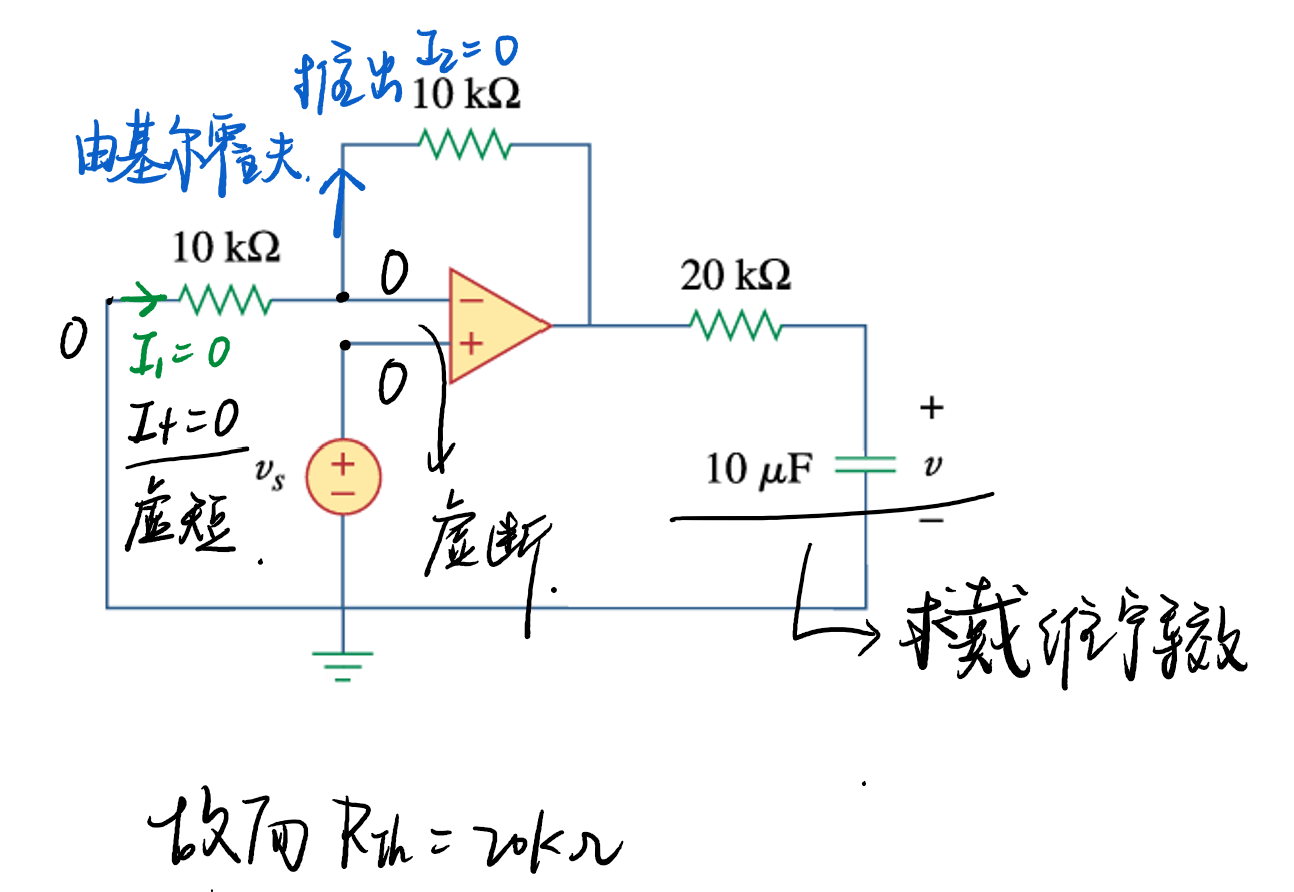
Thevenin equivalent-solve quadratic equation
Interesting problems
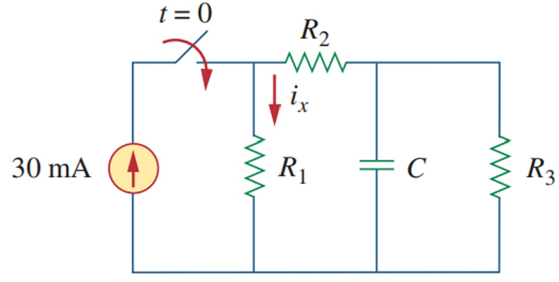
7.50 t = 0 t=0 t = 0 R 3 R_{3} R 3
when i 0 = 0 i_{0}=0 i 0 = 0
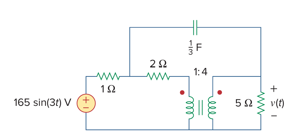
13.47 using mesh method.


 (using mesh method)
 (using nodal method)